Tutorial: Applying image filters

This tutorial describes how to apply image filters using MIRP.

Download example data

Here we use a publicly available chest CT dataset, that consist of a single image dataset and a mask.

from urllib.request import urlopen
from io import BytesIO
from zipfile import ZipFile

url = r"https://github.com/oncoray/mirp/raw/598293f7afb179b525b49f9b8300a9914fbdebd4/data/tutorial_radiomics_chest_ct_data.zip"

# Specify location where the data is stored.
save_dir = "."

with urlopen(url) as zip_url_pointer:
    with ZipFile(BytesIO(zip_url_pointer.read())) as example_data:
        example_data.extractall(save_dir)

This creates a folder with the following structure:

chest_ct
 ├─ image
 |  ├─ DCM_IMG_00000.dcm
 |  ├─ ...
 |  └─ DCM_IMG_00059.dcm
 └─ mask
    └─ DCM_RS_00060.dcm

In this example dataset, the CT image slices are stored in DICOM format in the image directory. A segmentation mask is stored in DICOM format in the mask subdirectory.

Finding mask labels

Radiomics features are typically computed from regions of interest, such as a tumour. These regions are delineated by experts or auto-segmentation AI, and stored as segmentation masks. MIRP needs to know which mask label (region of interest) should be used for computing features. A first step is to identify which mask labels exist. This can be done using the extract_mask_labels function. In this example, we directly provide a path to the mask file (.../chest_ct/mask/DCM_RS_00060.dcm).

import os
from mirp import extract_mask_labels

extract_mask_labels(
    mask=os.path.join(save_dir, "chest_ct", "mask", "DCM_RS_00060.dcm"),
)

	sample_name	modality	dir_path	file_name	series_instance_uid	frame_of_reference_uid	roi_label	mask_index
0	1	rtstruct	.\chest_ct\mask	DCM_RS_00060.dcm	1.3.6.1.4.1.9590.100.1.2.258301620411152643708...	1.3.6.1.4.1.9590.100.1.2.437537500115184941017...	GTV-1	0

The mask file contains only a single mask, called GTV-1.

Visualising images

It is often useful to inspect images before computing radiomics features. External viewers for DICOM and many other image types exist, but MIRP also has a simple visualisation tool. You can visualise images by exporting them in MIRP internal formats using extract_images:

from mirp import extract_images

images = extract_images(
    image=os.path.join(save_dir, "chest_ct", "image"),
    mask=os.path.join(save_dir, "chest_ct", "mask", "DCM_RS_00060.dcm"),
    roi_name="GTV-1",
    image_export_format="native"
)

INFO    : MainProcess    2024-06-18 08:26:19,447         Initialising image extraction using ct images for 1.

By default, extract_images will export dictionaries containing image and mask data (as numpy.ndarray) and associated metadata. That way extract_images can be used to read and process images as part of an external workflow. The default output can be visualised using matplotlib and other tools. Here we use image_export_format="native" to export images and masks in the native MIRP format. The output of extract_images is a list of images and masks, with one entry per image dataset. We only assess a single image here, which means that images only has one element. The nested list always consists of the image – and any derivatives, such as filtered images – and masks associated with the image. We can visualise an exported image using its show method as follows:

image, mask = images[0]
image[0].show(mask=mask[0], slice_id=25)

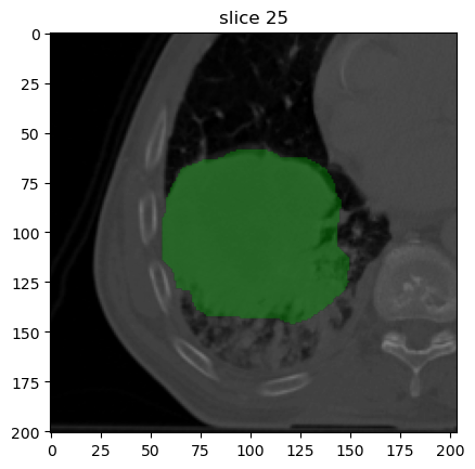
Though just an image is shown here, executing this code outside of a Jupyter Notebook will start an interactive plotter that can be scrolled through.

The CT image appears as expected: a large solid tumour is located in the right lung lobe.

Assessing image metadata

Image metadata are important for understanding the image and how it was acquired and reconstructed. MIRP allows for exporting image metadata from DICOM and other image formats, though for non-DICOM formats metadata will be considerably more limited.

from mirp import extract_image_parameters

extract_image_parameters(
    image=os.path.join(save_dir, "chest_ct", "image")
)

	sample_name	modality	dir_path	spacing_z	spacing_y	spacing_x	file_name	series_instance_uid	frame_of_reference_uid	scanner_type	manufacturer	image_type	image_index
0	1	ct	chest_ct\image	3.0	0.977	0.977	DCM_IMG_00059.dcm	1.3.6.1.4.1.9590.100.1.2.296658988911737913102...	1.3.6.1.4.1.9590.100.1.2.437537500115184941017...	CERR	CMS, Inc.	['ORIGINAL', 'PRIMARY', 'AXIAL']	0

Only known metadata are shown. For example, tube voltage was not present in the image metadata in this example.

The metadata, and our use case, have important implications for the image processing:

• Since we want to apply filters, we should ensure that pixel or voxel spacing should be isotropic.

• The in-plane resolution is a bit higher than the distance between slices, but can be resampled to isotropic voxels, e.g. 1.0 by 1.0 mm by 1.0 mm. We can apply a filter in 3D.

Applying filters

Image filters can be used to enhance specific characteristics of an image. Here we will apply to three filters: a mean filter, a Laplacian-of-Gaussian filter, and a non-separable wavelet filter. To do so, we specify the following parameters:

1. Voxels are resampled to 1.0 by 1.0 by 1.0 mm (new_spacing=1.0).

2. Select filters (filter_kernels=["mean", "laplacian_of_gaussian", "nonseparable_wavelet"])

3. Set width of the mean filter (in voxels) (mean_filter_kernel_size=5).

4. Set width of the Laplacian-of-Gaussian filter (in mm) (laplacian_of_gaussian_sigma=[1.0, 3.0]). Here we apply two filters: one with σ = 1.0 mm, and one with σ = 3.0.

5. Use the Simoncelli wavelet (nonseparable_wavelet_families="simoncelli").

6. Find the first three decompositions of the Simoncelli wavelet (nonseparable_wavelet_decomposition_level=[1, 2, 3]).

Many more parameters can be specified, see Configure the image processing and feature extraction workflow.

from mirp import extract_images

images = extract_images(
    image=os.path.join(save_dir, "chest_ct", "image"),
    mask=os.path.join(save_dir, "chest_ct", "mask", "DCM_RS_00060.dcm"),
    roi_name="GTV-1",
    image_export_format="native",
    new_spacing=1.0,
    filter_kernels=["mean", "laplacian_of_gaussian", "nonseparable_wavelet"],
    mean_filter_kernel_size=5,
    laplacian_of_gaussian_sigma=[1.0, 3.0],
    nonseparable_wavelet_families="simoncelli",
    nonseparable_wavelet_decomposition_level=[1, 2, 3]
)
image, mask = images[0]

INFO    : MainProcess    2024-06-18 08:26:22,640         Initialising image extraction using ct images for 1.

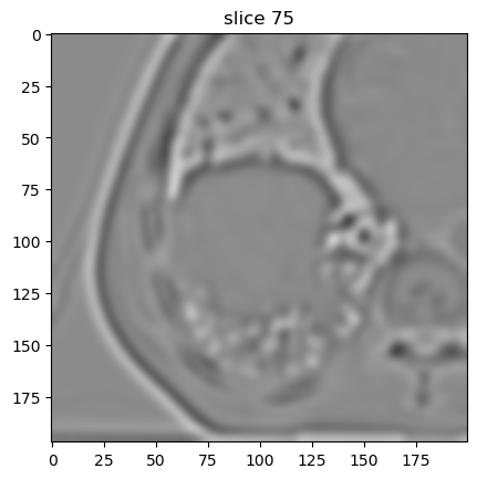
Now we can first plot the base image. The base image is always part of the export. Because we resampled the image slices from 3.0 to 1.0 mm, the number of slices increased compared to the original image.

image[0].show(slice_id=75)

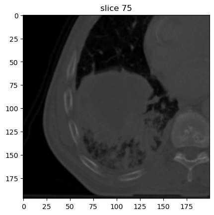
Derivative (i.e. filtered) images are stored in the same list as the base image (image[0]).

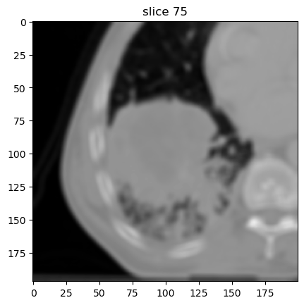
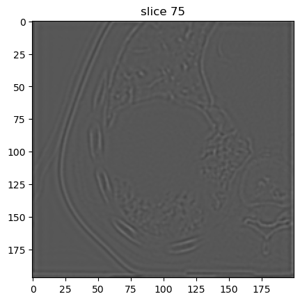
Mean filter

image[1].show(slice_id=75)

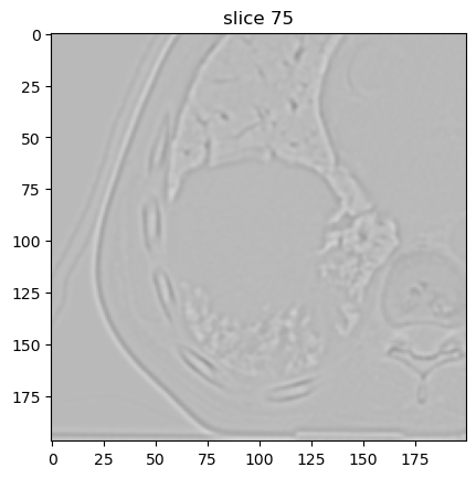
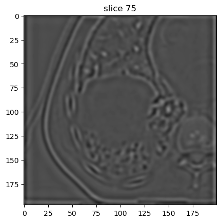
Laplacian-of-Gaussian filter

With σ = 1.0 mm:

image[2].show(slice_id=75)

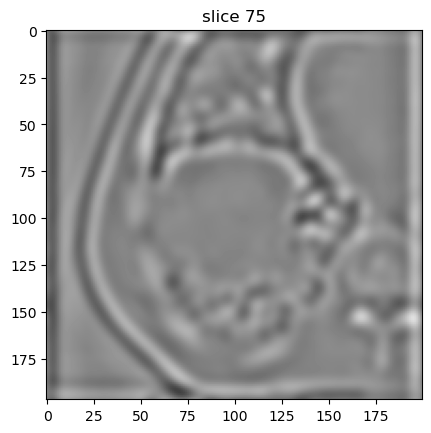
With σ = 3.0 mm:

image[3].show(slice_id=75)

Nonseparable Simoncelli wavelet filter

First decomposition level:

image[4].show(slice_id=75)

Second decomposition level:

image[5].show(slice_id=75)

Third decomposition level:

image[6].show(slice_id=75)

Computing features

Features can also be computed from filtered images. By default, only statistical features are computed, in addition to features computed from the base image.

For the base image, we need to define parameters related to intensity discretisation for computing histogram-based and texture features. Since a CT image consists of Hounsfield units (HU), which are typically calibrated, we will use a fixed bin size algorithm (base_discretisation_method="fixed_bin_size") with a bin size of 20 HU (base_discretisation_bin_size=20.0). This method requires setting the lowest intensity of the first bin. By default, MIRP uses -1000 HU (corresponding to air). However, this is not always the most useful setting. Here, we will instead specify a soft-tissue window (resegmentation_intensity_range=[-180.0, 200.0]), which sets the lowest intensity of the first bin to -180 HU.

import pandas as pd
from mirp import extract_features

features = extract_features(
    image=os.path.join(save_dir, "chest_ct", "image"),
    mask=os.path.join(save_dir, "chest_ct", "mask", "DCM_RS_00060.dcm"),
    roi_name="GTV-1",
    image_export_format="native",
    new_spacing=1.0,
    resegmentation_intensity_range=[-180.0, 200.0],
    base_discretisation_method="fixed_bin_size",
    base_discretisation_bin_width=20.0,
    filter_kernels=["mean", "laplacian_of_gaussian", "nonseparable_wavelet"],
    mean_filter_kernel_size=5,
    laplacian_of_gaussian_sigma=[1.0, 3.0],
    nonseparable_wavelet_families="simoncelli",
    nonseparable_wavelet_decomposition_level=[1, 2, 3]
)

pd.concat(features)

INFO    : MainProcess    2024-06-18 08:26:38,268         Initialising feature computation using ct images for 1.

	sample_name	image_file_name	image_directory	image_study_date	image_study_description	image_series_description	image_series_instance_uid	image_modality	image_pet_suv_type	image_mask_label	...	wavelet_simoncelli_level_3_stat_max	wavelet_simoncelli_level_3_stat_iqr	wavelet_simoncelli_level_3_stat_range	wavelet_simoncelli_level_3_stat_mad	wavelet_simoncelli_level_3_stat_rmad	wavelet_simoncelli_level_3_stat_medad	wavelet_simoncelli_level_3_stat_cov	wavelet_simoncelli_level_3_stat_qcod	wavelet_simoncelli_level_3_stat_energy	wavelet_simoncelli_level_3_stat_rms
0	1	None	chest_ct\image	None	None	None	1.3.6.1.4.1.9590.100.1.2.296658988911737913102...	ct	None	GTV-1	...	531.404254	77.65685	863.020984	61.349115	35.8172	58.114405	3.115791	2.045865	2.349373e+09	88.482671

1 rows × 311 columns

This results in a pandas.DataFrame that has a row per image and mask. The first several columns contain parameters related to that image and mask, and how these were processed. The features computed from filtered images are appended after the features from the base image. These features can be used for, e.g., machine learning using scikit-learn or familiar.