Tutorial: Computing radiomics features
This tutorial describes step-by-step how you can compute radiomics features from medical imaging using MIRP.
Download example data
We have prepared an (anonymised) example dataset of T1-weighted images of patients with soft-tissue sarcoma, that is a subset of the public Soft-tissue Sarcoma dataset [1]. The example dataset is a zip-file containing imaging data for three patients.
[2]:
from urllib.request import urlopen
from io import BytesIO
from zipfile import ZipFile

url = r"https://github.com/oncoray/mirp/raw/acd0b11521acd07aa9597e8f55d480bc54af4e04/data/tutorial_radiomics_mr_t1_data.zip"

# Specify location where the data is stored.
save_dir = "."

with urlopen(url) as zip_url_pointer:
    with ZipFile(BytesIO(zip_url_pointer.read())) as example_data:
        example_data.extractall(save_dir)
This creates a folder with the following structure:
sts_images
├─ STS_001
│   └─ ...
├─ ...
└─ STS_003
    └─ mr_t1
        ├─ image
        |  ├─ 1-01.dcm
        |  ├─ ...
        |  └─ 1-36.dcm
        └─ mask
            └─ 1-1.dcm
In this example dataset, the T1-weighted images are stored in DICOM format in the mr_t1/image subdirectory. A segmentation mask is also stored in DICOM format, but in the mr_t1/mask subdirectory.
Finding mask labels
Radiomics features are typically computed from regions of interest, such as a tumour. These regions are delineated by experts or auto-segmentation AI, and stored as segmentation masks. MIRP needs to know which mask label (region of interest) should be used for computing features. A first step is to identify which mask labels exist. This can be done using the extract_mask_labels function. We need to define the main directory (.../sts_images), and optionally the directory structure
relative to the patient directory (mr_t1/mask), where the masks can be found.
[3]:
import os
from mirp import extract_mask_labels

extract_mask_labels(
    mask=os.path.join(save_dir, "sts_images"),
    mask_sub_folder=os.path.join("mr_t1", "mask")
)
[3]:
| sample_name | modality | dir_path | file_name | study_description | series_description | acquisition_time | series_instance_uid | frame_of_reference_uid | roi_label | mask_index | |
|---|---|---|---|---|---|---|---|---|---|---|---|
| 0 | STS_001 | rtstruct | sts_images\STS_001\mr_t1\mask | 1-1.dcm | ^THIGH | RTstruct_T1 | 2009-10-17 17:16:35.000915 | 1.3.6.1.4.1.14519.5.2.1.5168.1900.169505605471... | 1.3.6.1.4.1.14519.5.2.1.5168.1900.178691248814... | GTV_Mass | 0 |
| 1 | STS_001 | rtstruct | sts_images\STS_001\mr_t1\mask | 1-1.dcm | ^THIGH | RTstruct_T1 | 2009-10-17 17:16:35.000915 | 1.3.6.1.4.1.14519.5.2.1.5168.1900.169505605471... | 1.3.6.1.4.1.14519.5.2.1.5168.1900.178691248814... | GTV_Edema | 0 |
| 0 | STS_002 | rtstruct | sts_images\STS_002\mr_t1\mask | 1-1.dcm | L-SPINE | RTstruct_T1 | 2009-10-18 11:56:49.000312 | 1.3.6.1.4.1.14519.5.2.1.5168.1900.337975716601... | 1.3.6.1.4.1.14519.5.2.1.5168.1900.188414386222... | GTV_Mass | 1 |
| 1 | STS_002 | rtstruct | sts_images\STS_002\mr_t1\mask | 1-1.dcm | L-SPINE | RTstruct_T1 | 2009-10-18 11:56:49.000312 | 1.3.6.1.4.1.14519.5.2.1.5168.1900.337975716601... | 1.3.6.1.4.1.14519.5.2.1.5168.1900.188414386222... | GTV_Edema | 1 |
| 0 | STS_003 | rtstruct | sts_images\STS_003\mr_t1\mask | 1-1.dcm | MRI PELVIS C- C | RTstruct_T1 | 2009-10-18 12:10:34.000164 | 1.3.6.1.4.1.14519.5.2.1.5168.1900.200331945037... | 1.3.6.1.4.1.14519.5.2.1.5168.1900.179145981196... | GTV_Mass | 2 |
| 1 | STS_003 | rtstruct | sts_images\STS_003\mr_t1\mask | 1-1.dcm | MRI PELVIS C- C | RTstruct_T1 | 2009-10-18 12:10:34.000164 | 1.3.6.1.4.1.14519.5.2.1.5168.1900.200331945037... | 1.3.6.1.4.1.14519.5.2.1.5168.1900.179145981196... | GTV_Edema | 2 |
We are lucky that all masks are consistently labelled. GTV_Mass and GTV_Edema both refer to the gross tumour volume, i.e. that part of the tumour that is visible in medical imaging. GTV-Edema also covers fluid surrounding the gross tumour volume itself.
Visualising images
It is often useful to inspect images before computing radiomics features. External viewers for DICOM and many other image types exist, but MIRP also has a simple visualisation tool. You can visualise images by exporting them in MIRP internal formats using extract_images:
[4]:
from mirp import extract_images

images = extract_images(
    image=os.path.join(save_dir, "sts_images", "STS_003", "mr_t1", "image"),
    mask=os.path.join(save_dir, "sts_images", "STS_003", "mr_t1", "mask"),
    roi_name="GTV_Mass",
    image_export_format="native"
)
INFO : MainProcess 2024-06-20 17:08:52,671 Initialising image extraction using mr images for STS_003.
By default, extract_images will export dictionaries containing image and mask data (as numpy.ndarray) and associated metadata. That way extract_images can be used to read and process images as part of an external workflow. The default output can be visualised using matplotlib and other tools. Here we use image_export_format="native" to export images and masks in the native MIRP format. The output of extract_images is a list of images and masks, with one entry per image
dataset. We only assess a single image here, which means that images only has one element. The nested list always consists of the image – and any derivatives, such as filtered images – and masks associated with the image. We can visualise an exported image using its show method as follows:
[5]:
image, mask = images[0]
image[0].show(mask=mask[0], slice_id=10)
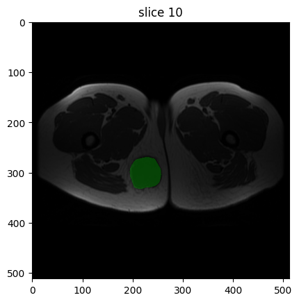
Though just an image is shown here, executing this code outside of a Jupyter Notebook will start an interactive plotter that can be scrolled through.
The T1-weighted image appears as expected: muscle tissue appears grey, and fatty tissue appears bright. The GTV_Mass segmentation mask covers the tumour – use image[0].show() to view the image without a mask.
Assessing image metadata
Image metadata are important for understanding the image and how it was acquired and reconstructed. MIRP allows for exporting image metadata from DICOM and other image formats, though for non-DICOM formats metadata will be considerably more limited.
[6]:
from mirp import extract_image_parameters

extract_image_parameters(
    image=os.path.join(save_dir, "sts_images"),
    image_sub_folder=os.path.join("mr_t1", "image")
)
[6]:
| sample_name | modality | dir_path | spacing_z | spacing_y | spacing_x | file_name | study_description | series_description | acquisition_time | series_instance_uid | frame_of_reference_uid | scanner_type | manufacturer | image_type | scanning_sequence | scanning_sequence_variant | image_index | |
|---|---|---|---|---|---|---|---|---|---|---|---|---|---|---|---|---|---|---|
| 0 | STS_001 | mr | sts_images\STS_001\mr_t1\image | 5.2 | 0.390625 | 0.390625 | 1-40.dcm | ^THIGH | AXIAL SE T1 - RESEARCH | 2000-09-03 11:10:33.000876 | 1.3.6.1.4.1.14519.5.2.1.5168.1900.236909650266... | 1.3.6.1.4.1.14519.5.2.1.5168.1900.178691248814... | Avanto | SIEMENS | ['ORIGINAL', 'PRIMARY', 'M', 'ND', 'NORM'] | SE | ['SK', 'SP', 'OSP'] | 0 |
| 1 | STS_002 | mr | sts_images\STS_002\mr_t1\image | 7.0 | 0.892857 | 0.892857 | 1-01.dcm | L-SPINE | AXT1 | 2006-01-03 14:19:40.000530 | 1.3.6.1.4.1.14519.5.2.1.5168.1900.103003228939... | 1.3.6.1.4.1.14519.5.2.1.5168.1900.188414386222... | Intera | Philips Medical Systems | ['ORIGINAL', 'PRIMARY', 'M_SE', 'M', 'SE'] | SE | OSP | 1 |
| 2 | STS_003 | mr | sts_images\STS_003\mr_t1\image | 7.0 | 0.781300 | 0.781300 | 1-36.dcm | MRI PELVIS C- C | AX T1 | 2005-03-30 11:28:05.000000 | 1.3.6.1.4.1.14519.5.2.1.5168.1900.900154069973... | 1.3.6.1.4.1.14519.5.2.1.5168.1900.179145981196... | Signa HDxt | GE MEDICAL SYSTEMS | ['ORIGINAL', 'PRIMARY', 'OTHER'] | SE | SK | 2 |
Only known metadata are shown. For example, magnetic field strength was not present in the image metadata in this example.
The metadata have important implications for the image processing:
The in-plane resolution is much higher than the distance between slices. This suggests that features should be computed by slice, instead in 3D.
The in-plane resolution differs between patients. This suggests that the images should be resampled to isotropic pixel sizes, e.g. 1.0 by 1.0 mm.
All three images were recorded in different scanners. This suggests that MR intensities cannot be compared between patients, and should be standardised.
Computing features
The presented metadata suggest that image processing is required to make the MR images more comparable between patients. We will define three image processing steps:
Image processing and feature computation are performed by slice (
by_slice=True) due to large distances between image slices.In-plane resolution is resampled to 1.0 by 1.0 mm (
new_spacing=1.0).Intensities are normalised, here using z-normalisation (
intensity_normalisation="standardisation").
In addition, we need to define parameters related to intensity discretisation for computing histogram-based and texture features. Since intensities were normalised using z-normalisation, we will use a fixed bin number algorithm (base_discretisation_method="fixed_bin_number") with 16 bins (base_discretisation_n_bins=16).
Many more parameters can be specified, see Configure the image processing and feature extraction workflow.
[7]:
import pandas as pd
from mirp import extract_features

features = extract_features(
    image=os.path.join(save_dir, "sts_images"),
    image_sub_folder=os.path.join("mr_t1", "image"),
    mask=os.path.join(save_dir, "sts_images"),
    mask_sub_folder=os.path.join("mr_t1", "mask"),
    roi_name="GTV_Mass",
    by_slice=True,
    intensity_normalisation="standardisation",
    new_spacing=1.0,
    base_discretisation_method="fixed_bin_number",
    base_discretisation_n_bins=16
)

pd.concat(features)
INFO    : MainProcess    2024-06-20 17:08:54,208         Initialising feature computation using mr images for STS_001.
INFO    : MainProcess    2024-06-20 17:09:07,088         Initialising feature computation using mr images for STS_002.
INFO    : MainProcess    2024-06-20 17:09:16,781         Initialising feature computation using mr images for STS_003.
[7]:
| sample_name | image_file_name | image_directory | image_study_date | image_study_description | image_series_description | image_series_instance_uid | image_modality | image_pet_suv_type | image_mask_label | ... | ngl_hdhge_d1_a0.0_2d_fbn_n16 | ngl_glnu_d1_a0.0_2d_fbn_n16 | ngl_glnu_norm_d1_a0.0_2d_fbn_n16 | ngl_dcnu_d1_a0.0_2d_fbn_n16 | ngl_dcnu_norm_d1_a0.0_2d_fbn_n16 | ngl_dc_perc_d1_a0.0_2d_fbn_n16 | ngl_gl_var_d1_a0.0_2d_fbn_n16 | ngl_dc_var_d1_a0.0_2d_fbn_n16 | ngl_dc_entr_d1_a0.0_2d_fbn_n16 | ngl_dc_energy_d1_a0.0_2d_fbn_n16 | |
|---|---|---|---|---|---|---|---|---|---|---|---|---|---|---|---|---|---|---|---|---|---|
| 0 | STS_001 | None | sts_images\STS_001\mr_t1\image | 20000903 | ^THIGH | AXIAL SE T1 - RESEARCH | 1.3.6.1.4.1.14519.5.2.1.5168.1900.236909650266... | mr | None | GTV_Mass | ... | 649.904779 | 685.643163 | 0.202679 | 573.379973 | 0.164149 | 1.0 | 2.124407 | 2.835808 | 5.207281 | 0.034652 |
| 0 | STS_002 | None | sts_images\STS_002\mr_t1\image | 20060103 | L-SPINE | AXT1 | 1.3.6.1.4.1.14519.5.2.1.5168.1900.103003228939... | mr | None | GTV_Mass | ... | 731.317187 | 232.044296 | 0.208755 | 212.059230 | 0.183419 | 1.0 | 3.301315 | 5.169630 | 5.048137 | 0.050158 |
| 0 | STS_003 | None | sts_images\STS_003\mr_t1\image | 20050330 | MRI PELVIS C- C | AX T1 | 1.3.6.1.4.1.14519.5.2.1.5168.1900.900154069973... | mr | None | GTV_Mass | ... | 608.689328 | 472.701740 | 0.345461 | 334.257475 | 0.238191 | 1.0 | 3.232402 | 5.422279 | 4.222418 | 0.132661 |
3 rows × 203 columns
This results in a pandas.DataFrame that has a row per image and mask. The first several columns contain parameters related to that image and mask, and how these were processed. After these, feature values are shown. These can be used for, e.g., machine learning using scikit-learn or familiar.
References
Vallières, Martin, Freeman, Carolyn R., Skamene, Sonia R., & El Naqa, Issam. (2015). A radiomics model from joint FDG-PET and MRI texture features for the prediction of lung metastases in soft-tissue sarcomas of the extremities (Soft-tissue-Sarcoma) [Dataset]. The Cancer Imaging Archive. http://doi.org/10.7937/K9/TCIA.2015.7GO2GSKS